§ 2.24 Immersed rotational shrinking spheres (Drugan, 2013; Drugan–Lee–X. H. Nguyen, 2017)2101D51F1E32

For each $n\geq 2$, there is a smooth rotational immersion $X:S^ n\to \mathbb R^{n+1}$ satisfying $\vec H=-X^\perp /2$ whose image is not embedded. The associated immersed flow is $X_ t=\sqrt{-t}\, X$, $-\infty <t<0$. In the three-dimensional construction, a graphical piece of the profile, written as axial height $z=\gamma (r)$ for $r>0$, solves

This is equation (1.2) of [Drugan2015], p. 3140; the paper's radial variable $x$ is denoted here by $r$. Equation (1.3) describes the same curve as a radius depending on height. Shooting and continuation through profile turning points produce the closed immersed sphere; a single graphical piece does not describe the whole surface.

• The parameter domain is the compact sphere, so the induced metric is complete and the immersion is proper. The image has self-intersections and is not the round sphere.

• The construction has rotational symmetry and reflection symmetry across a hyperplane perpendicular to the rotation axis. It has no ends. The homothetic flow contracts to the origin with Type I curvature growth.

• The cited existence argument supplies neither an elementary parametrization nor uniqueness or an exact entropy value. Embedded classification and embedded stability theorems cannot be applied to this immersion by dropping their embeddedness hypothesis.

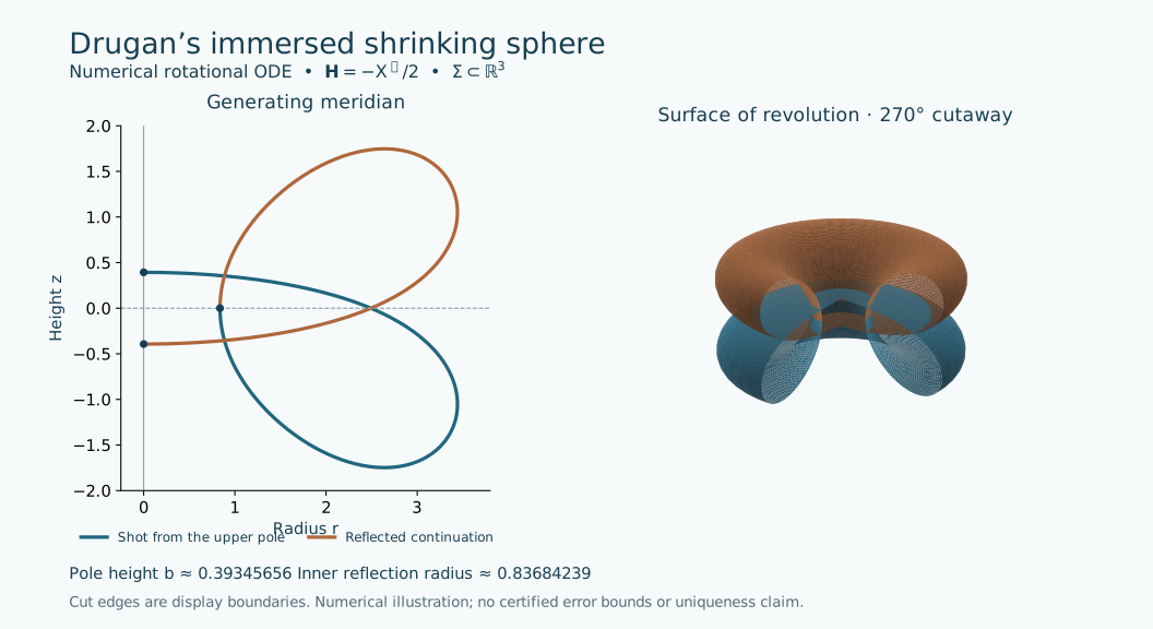
Numerical picture. The picture computes the rotational shooting construction in [Drugan2015], Sections 2–5, and can be compared with Figure 1 on p. 3141. It shows the two-dimensional immersed sphere in $\mathbb R^3$, not a higher-dimensional projection. Let $s$ be arc length along the meridian and let $\theta $ be its tangent angle measured from the positive radial direction. Substituting $\gamma '=\tan \theta $ into the graph equation gives

This system continues through the vertical tangents where the graph equation becomes unsuitable for numerical integration. At the upper pole $(r,z)=(0,b)$, smoothness requires $\theta =0$. The even expansion from the graph equation, consistent with Section 6 of the paper, is

We start at $r=10^{-4}$ using this expansion and shoot in $b$ until $z=0$ at the second radial turning point, where $\theta =-3\pi /2$. This is the orthogonal reflection condition in Section 5, pp. 3154–3155. The computation gives

Reflection across $z=0$, with the order of traversal reversed, completes the meridian from $(0,b)$ to $(0,-b)$. Revolving it gives

with the angular circles collapsed at the two poles. This is a numerical parametrization at time $t=-1$; the corresponding flow is $X_ t=\sqrt{-t}\, X$ for $t<0$.

The meridian view shows the self-intersections directly. The revolution angle control reveals interior sheets by removing angular sectors; the resulting cut edges are display boundaries, not boundaries of the immersed sphere. The two colors distinguish the shot half from its reflected continuation. The shooting height residual is below $10^{-10}$ before rounding the exported mesh. Halving the initial radius and maximum step and tightening the integration tolerances changes the computed pole height and reflection radius by less than $10^{-9}$. These are floating-point convergence diagnostics, not certified error bounds. In particular, numerical shooting does not prove existence, uniqueness, or that this root is the supremum used in Drugan's proof.