MCF-stack: Special Solutions of Mean Curvature Flow

§ 5.37 Su–Wood stationary products of Lawlor profilesC99B5440B24D

Earliest recorded reference: (first arXiv submission).

Paper credits and chronology

Paper credits are chronological and include every author of the cited papers. They identify sources, not exclusive discovery credit. Background-only citations do not determine the date of this example. A classical example may predate the references recorded here.

  1. Su–Wood — 2025-07-02 (first arXiv submission).
C99B5440B24D
3CC118326D79

(Cohomogeneity-two special Lagrangians) Let $m\geq 3$, $d=m-1$, $I=(-\pi /(2d),\pi /(2d))$, $\mu _1,\mu _2>0$, and $\varphi \in \mathbb R$. Define

\[ r(s)=(\cos (ds))^{-1/d},\quad \ell (s)=r(s)e^{is},\quad B(s)=\int _0^ s r(v)^2\, dv. \]

For $u\in S^{m-2}\subset \mathbb R^{m-1}$ and $(x,y)\in I^2$, put

\[ X(u,x,y)=\left(e^{i\varphi }\mu _1\mu _2\ell (x)\ell (y)u, \frac{\mu _2^2r(y)^2-\mu _1^2r(x)^2}{2} +i\bigl (\mu _2^2B(y)-\mu _1^2B(x)\bigr )\right)\in \mathbb C^ m. \]

This is an exact integral parametrization of an embedded, exact special Lagrangian of dimension and codimension $m$. Thus $\vec H=0$ and $L_ t=X(S^{m-2}\times I^2)$ for every $t\in \mathbb R$. It is the $G=SO(m-1)$ case of [SuWood2026], equation (31), Theorem 5.6, Proposition 5.9 and Remark 5.10. It has cohomogeneity two under this group; for $m=3$ the topology is $S^1\times \mathbb R^2$, not a surface annulus.

The topology in general is $S^{m-2}\times \mathbb R^2$, with one end. The parametrization is proper: approaching either endpoint of $I$ makes $|\ell (x)\ell (y)|$ diverge, and the remaining factor $u$ is compact. The induced metric is therefore complete. The calibrated image is stable under compactly supported variations. No entropy value or global asymptotic classification is recorded here.

For the illustrated case $m=3$, write $s=\arctan (\tanh q)$. Then

\[ \ell (s)=\cosh q+i\sinh q,\qquad B(s)=q. \]

Thus equation (31) has a closed elementary form in this dimension. Fix $\mu _1=1$, $\mu _2=\mu >0$, and $\varphi =0$. For $(p,b)\in \mathbb R^2$, set $a=\operatorname {arsinh}p$ and

\[ Z=\mu (\cosh b+ip),\qquad W=\frac{\mu ^2\cosh (a+b)-\cosh (a-b)}2 +\frac{i}{2}\bigl ((\mu ^2-1)a+(\mu ^2+1)b\bigr ). \]

The full stationary flow is

\[ X_ t(\theta ,p,b)=(Z\cos \theta ,Z\sin \theta ,W)\in \mathbb C^3, \qquad \theta \in \mathbb R/(2\pi \mathbb Z),\quad t\in \mathbb R. \]

This is a reparametrization of the displayed construction, obtained by putting the two hyperbolic profile parameters equal to $(a-b)/2$ and $(a+b)/2$. For $\mu =1$, the profile projection is particularly simple:

\[ (\operatorname {Im}Z,\operatorname {Re}W,\operatorname {Im}W) =(p,p\sinh b,b),\qquad \operatorname {Re}Z=\cosh b. \]

The figure samples these exact formulas on $|p|\leq 2$, $|b|\leq 1.2$. The snapshots at $t=-2,0,2$ coincide, including their spatial scale and marked parameter point: $\partial _ tX_ t=\vec H=0$. The circle view adds sampled spatial $SO(2)$ orbits. Changing $\mu $, the orbit angle, or the projection changes the example or its view, not its mean curvature flow. The colored sheet is a two-dimensional profile, not the entire three-manifold and not a surface mean curvature flow in $\mathbb R^3$.

The same paper constructs translators from a line and an Anciaux shrinker profile, and from an expander/shrinker pair. The line/expander case recovers the symmetric Joyce–Lee–Tsui translator of Example 3.17; it is not a second catalogue entry. For other symmetry groups some constructions have a one-dimensional singular set, so their smooth embeddedness must not be inferred from this $SO(m-1)$ case.
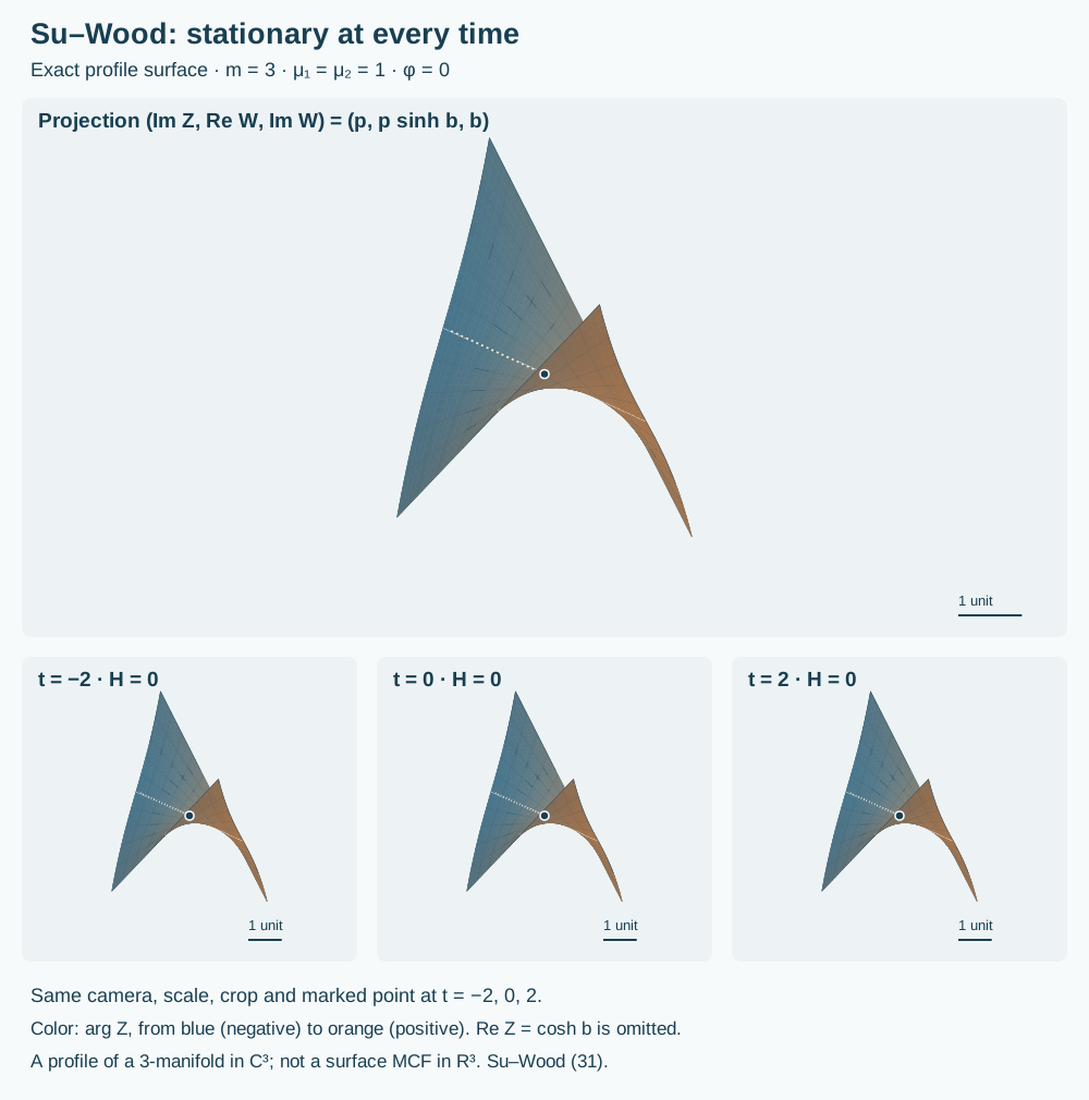
An exact projected Su–Wood profile surface with identical snapshots at times −2, 0 and 2. The full stationary special Lagrangian has dimension three in C³.
Exact formula; projected profile and circle orbits. The m = 3, SO(2) family from Su–Wood (31), evaluated in closed form. Three identical time panels show Lₜ = L₀, since H = 0. The profile view projects a two-dimensional surface in C²; the circle view reconstructs selected leaves and orbits of the three-manifold in C³. μ₁ = 1 and φ = 0; μ₂ changes the example, not time. Noncompact geometry is truncated. Color records arg Z; projection crossings do not imply self-intersections. Open drawing · Numerical references and credits

Ambient space, topology, embeddedness and entropy

Full Euclidean ambient dimension is 2m, at least six. The interactive figure uses the exact m = 3 formula, a projected two-dimensional profile, and sampled SO(2) orbits in R6. Every flow time has identical geometry. Neither the profile nor its projection determines a surface genus for this higher-dimensional example.

SO(m − 1)-invariant stationary examples in Cᵐ, m ≥ 3 · Euclidean dimension ≥ 5 · Embedded
Ambient space
Euclidean dimension ≥ 5
Topology
Sᵐ⁻² × R²
Embeddedness
Embedded: Embedded for this explicitly restricted case; no claim about other weights, groups, or singular limits.
Compactness
Noncompact
Surface genus
Intrinsic dimension at least three; surface genus is inapplicable.
Topological ends
One end; this is not a product of two complete Lawlor neck manifolds.
Entropy
Not recorded: No value or bound recorded from the checked source; entropy is not inferred from a single centered Gaussian integral.
Gaussian area
Not recorded: No value or bound recorded from the checked source; entropy is not inferred from a single centered Gaussian integral.

Compare examples by these properties →

References on this page

  1. [SuWood2026] Wei-Bo Su and Albert Wood. Lagrangian translating solitons and special lagrangians in cm with symmetries. 2026. Reviewed edition 2507.01345v1; selected statements checked. URL: https://arxiv.org/abs/2507.01345v1.All uses in this project ↩ 1
Cite this page

Comments

Comments are not enabled yet.