MCF-stack: Special Solutions of Mean Curvature Flow

§ 5.46 Lagrangian sphere chains in Gibbons–Hawking spaces2AB1CBD37191

Earliest recorded reference: (first arXiv submission).

Paper credits and chronology

Paper credits are chronological and include every author of the cited papers. They identify sources, not exclusive discovery credit. Background-only citations do not determine the date of this example. A classical example may predate the references recorded here.

  1. Lee–Tsai — 2026-06-27 (first arXiv submission).
2AB1CBD37191 These are surface flows of codimension two in a hyperkahler four-manifold.
DE8829990703

(Infinite-time curvature blow-up with vanishing mean curvature) Use the Gibbons–Hawking setting of [LeeTsai2026], Section 2: the circle quotient contains the collinear centers $(a_ j,0,0)$ with $-1=a_1<\cdots <a_ N=1$, $N\geq 3$, and

\[ \varphi =\varphi _{\rm reg}+\frac12\sum _{j=1}^ N ((x-a_ j)^2+y^2+z^2)^{-1/2},\qquad g=\varphi ^{-1}\eta ^2+\varphi (dx^2+dy^2+dz^2), \quad d\eta =*d\varphi . \]

The regular part is smooth, nonnegative, and harmonic on the source's quotient neighborhood. Let the initial Lagrangian sphere be the smooth circle lift of a positive concave graph $(x,u_0(x),0)$ joining the outer centers, with $u_0(\pm 1)=0$. For fixed $\Lambda >0$, require the small-slope and curvature conditions of Theorem 6.2:

\[ |u_0'|\leq c^{-1},\qquad -u_0''\leq \Lambda u_0\varphi (x,u_0,0), \]

where $c$ is sufficiently large as supplied by that theorem. The reduced equation is

\[ u_ t=\frac{u_{xx}}{\varphi (x,u,0)(1+u_ x^2)},\qquad u(\pm 1,t)=0. \]

The lifted flow exists smoothly for $t\geq 0$, remains a compact embedded sphere, and converges to the $A_{N-1}$ chain of $N-1$ special Lagrangian spheres. Theorem 6.2 proves

\[ \sup |\vec H|\longrightarrow 0,\qquad 0<\liminf _{t\to \infty }\frac{\log \max |A|}{\sqrt t} \leq \limsup _{t\to \infty }\frac{\log \max |A|}{\sqrt t}<\infty . \]

Finite-time slices have genus zero, no ends, and are complete and proper. Junctions occur only in the infinite-time limit. The quotient evolves by the weighted equation above, not ordinary planar curve shortening; Euclidean entropy is inapplicable. The coauthor is Ping-Hung Lee, distinct from Tang-Kai Lee.

The illustration integrates the quotient PDE numerically for $N=4$, $a_ j=-1+2(j-1)/3$, $\varphi _{\rm reg}=0$, and $u_0(x)=0.06(1-x^2)$, on $0\leq t\leq 12$. Its finite-time snapshots are separate from the theoretical limit $t\to \infty $. Mesh refinement checks numerical consistency; the chosen initial coefficient is not certified against the existential smallness constant in Theorem 6.2.

To interpret the diagram, the circle over $(x,u(x,t),0)$ has radius factor

\[ r_{\rm orb}(x,t)=\varphi (x,u(x,t),0)^{-1/2}. \]

The rendered surface $(x,r_{\rm orb}\cos \theta ,r_{\rm orb}\sin \theta )$, $0\leq \theta <2\pi $, records these fiber sizes; it is not an isometric embedding of $L_ t$ in Euclidean three-space. The outer fibers collapse at every time, closing a sphere. The two interior fibers stay positive at finite times. In the limit, each interval $[a_ j,a_{j+1}]$ lifts to a special Lagrangian sphere, with adjacent spheres meeting transversely in the four-manifold. The displayed contact angles have no geometric meaning. Remark 6.3 relates the neck size to $\| u(\cdot ,t)\| _{C^0}^{1/2}$ and to $(\max |A|)^{-1}$, explaining why small quotient height accompanies large curvature.
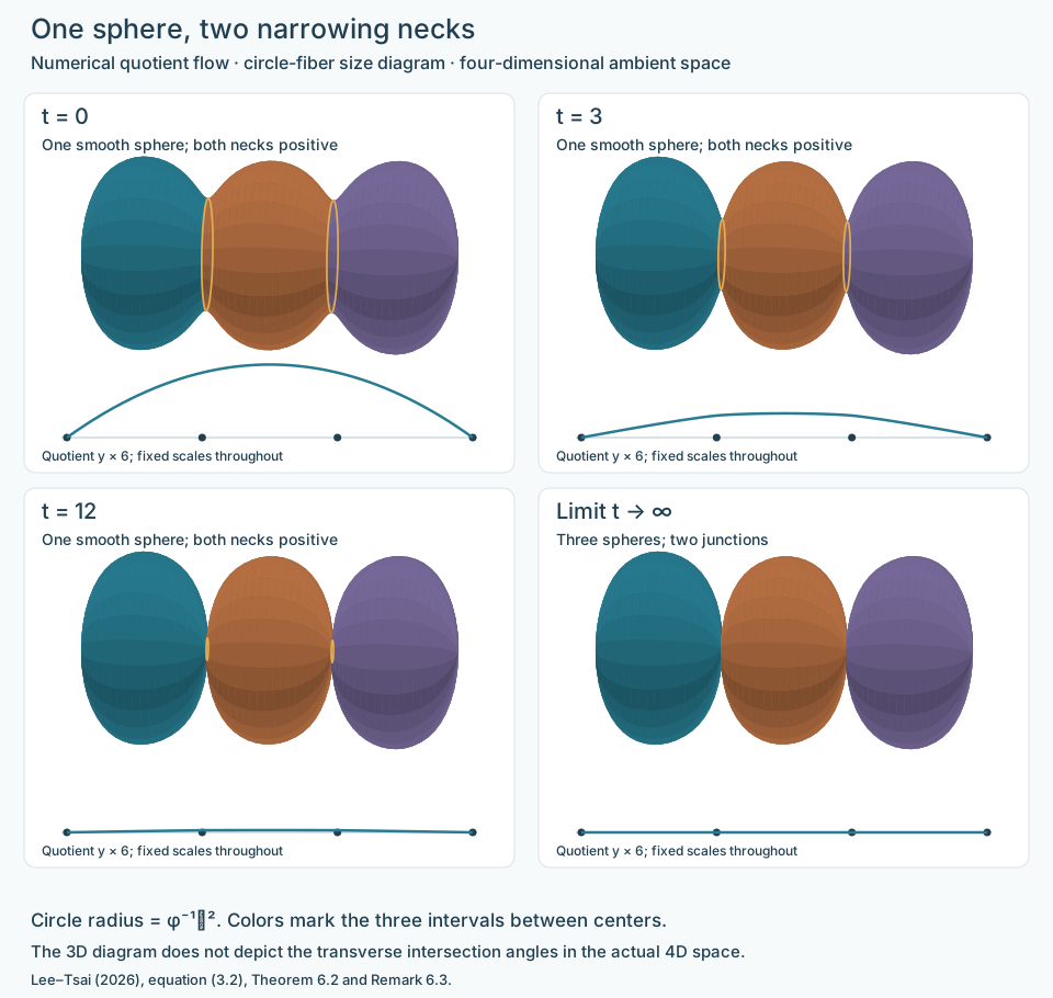
Numerical quotient profiles and circle-fiber size diagrams at t = 0, 3 and 12, alongside a separate infinite-time chain. Two positive necks narrow while the finite-time surface stays a sphere.
Numerical quotient flow and circle-fiber diagram. Four centers at −1, −1/3, 1/3, 1, with φreg = 0 and u(x,0) = 0.06(1 − x²). Compare t = 0, 3, 12, play the finite-time flow, or view the separate limit. Quotient height is magnified ×6. The colored surface plots circle radius φ⁻¹ᐟ² along x; it is a fiber-size diagram, not an isometric embedding in R³. Finite times show one sphere; the limiting three spheres intersect transversely in the actual four-manifold. The computation does not certify the theorem’s existential smallness threshold. Open drawing · Numerical references and credits

Ambient space, topology, embeddedness and entropy

Dimensions, topology, and embeddedness refer to the stated full ambient geometry and regular slices. See the source hypotheses and illustration conventions on this page.

Circle-invariant Lagrangian sphere in a hyperkähler four-manifold · Riemannian ambient manifold · Embedded
Ambient space
Riemannian ambient manifold
Topology
Sphere S² at every finite time; limiting A_(N−1) chain has N−1 spheres, N ≥ 3.
Embeddedness
Embedded: The positive quotient graph lifts to an embedded sphere; junctions of the limiting chain occur only at infinite time.
Compactness
Compact
Surface genus
0 for each finite-time sphere.
Topological ends
No ends (compact).
Entropy
Not applicable: Intrinsic mean curvature flow in a Riemannian ambient manifold; Euclidean Gaussian area and entropy are not assigned.
Gaussian area
Not applicable: Intrinsic mean curvature flow in a Riemannian ambient manifold; Euclidean Gaussian area and entropy are not assigned.

Compare examples by these properties →

References on this page

  1. [LeeTsai2026] Ping-Hung Lee and Chung-Jun Tsai. Infinite-time singularities with vanishing mean curvature for lagrangian mean curvature flow in gibbons–hawking spaces. 2026. Reviewed arXiv edition 2606.28767v1. Sections 2–3 for ambient metric and quotient PDE; Theorem 6.2 and its proof for precise initial slope/concavity hypotheses, N ≥ 3, vanishing H and log curvature / sqrt(t) bounds. URL: https://arxiv.org/abs/2606.28767v1.All uses in this project ↩ 1
Cite this page

Comments

Comments are not enabled yet.