41748F7ED1C1
(Prescribed Type II blow-up rates) For $n\geq 4$ and every integer $K\geq 2$, and for $n=3$ with $K\in \{ 2,3,4\} $, [StolarskiSu2026], Theorem 1.1 and Remark 1, construct smooth noncompact properly embedded exact almost-calibrated Lagrangian mean curvature flows $L(t)\subset \mathbb C^ n$, $0\leq t<T<\infty $. Here we record the $SO(n)$-invariant subfamily, of dimension and codimension $n$. Its topology is $S^{n-1}\times \mathbb R$, with two ends, and every regular slice is complete. The topology follows from the global profile graph and its spherical group orbits.
The origin is a finite-time Type II singularity with
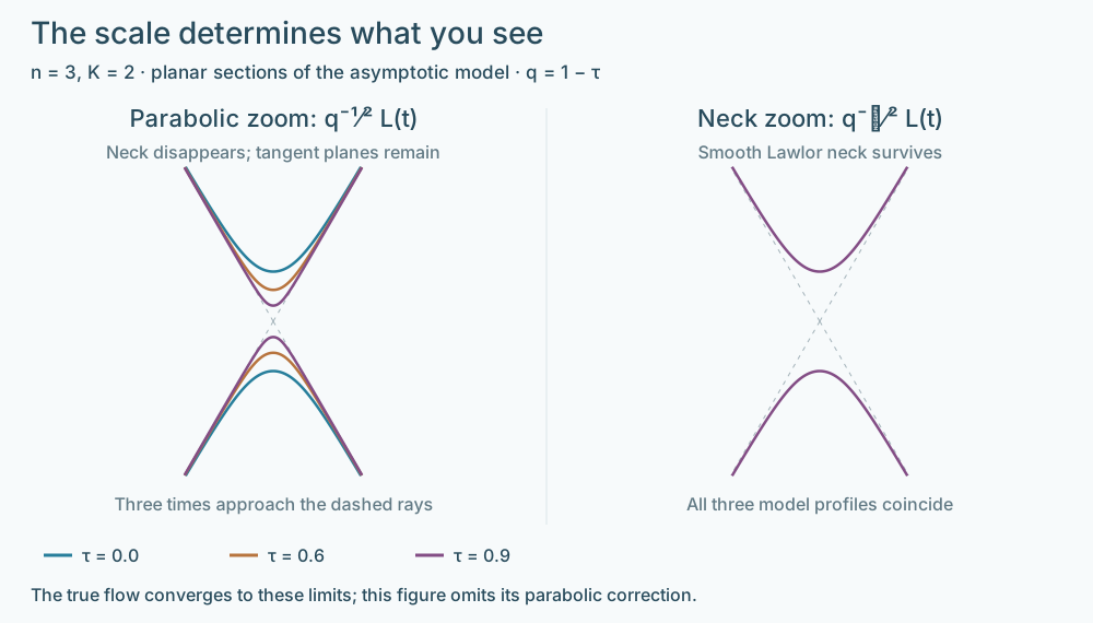
The unique tangent flow is a stationary multiplicity-one pair of transverse special Lagrangian planes. In contrast, the finer rescaling satisfies
where $L$ is the rotational Lawlor neck. Up to a fixed unitary rotation, that limiting neck has the exact parametrization
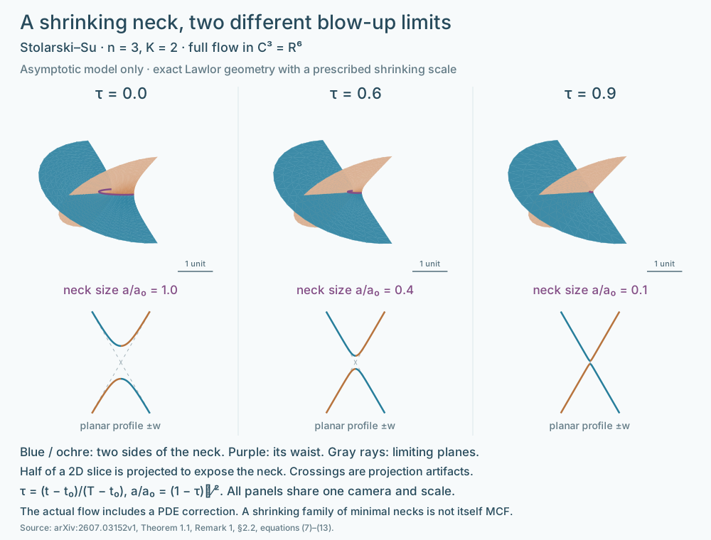
This is a formula for the blow-up limit, not for $L(t)$. The actual flow is constructed by solving a nonlinear parabolic problem near a modulated neck of scale comparable to $(T-t)^{K/2}$, and has no closed formula. The initial Lagrangian angle oscillation can be arbitrarily small. These existence and convergence statements do not assert dynamical stability, uniqueness of the initial data, or a numerical entropy value. The illustration uses the exact Lawlor profile above with a prescribed scale to show the near-singularity dynamics. With a reference time $t_0<T$, write
Here $a_0$ and the equality defining $a_{\mathrm{model}}$ are choices for the drawing, not an exact formula for the modulation parameter of the flow. The actual profile includes a correction obtained by solving the parabolic equation; see [StolarskiSu2026], Theorem 1.1(3) and Sections 2.2–2.3. A shrinking family of these minimal necks alone does not solve mean curvature flow.
The time comparison keeps the same spatial scale. Under parabolic magnification by $q^{-1/2}$ the model neck has scale $a_0q^{(K-1)/2}\to 0$; under the finer magnification by $q^{-K/2}$ its scale remains $a_0$. These illustrate the distinct tangent-plane and smooth-neck limits. The surface view restricts the spherical orbit to $u=(\cos \phi ,\sin \phi ,0,\ldots ,0)$ and projects this two-dimensional slice from $\mathbb C^2$ into $\mathbb R^3$. Projection may create apparent intersections. The planar view shows the exact profiles and their limiting rays. None of these drawings is a numerical time integration or a continuation through $T$. The compact immersed variant mentioned in the source's Remark 3 is outside this entry.
Comments
Comments are not enabled yet.